1. Introduction

The thought of surface energy balance has been exten-sively applied for various purposes especially in micro- meteorological analysis of phenomena relating to management of the Earth' resources. Carson (1982) has given a com-prehensive review of land-surface and the atmospheric boundary schemes used in many general circulation models with an emphasis on surface processes. Schmugge and Humes (1995) applied the surface energy balance model to monitor land surface fluxes. Many studies used Bowen ratio between sensible and latent heat fluxes to estimate the evapolation rate through surface energy balance equation (Brutsaert, 1982; Gutierres et al., 1994). Other papers deal with specific topics in more details, including Zhihao et al. (2002), Du et al. (2013), Lagos et al. (2011), Senay et al. (2010), Sato (2009).

The inclusion of soil surface and road condition is very important in an attempt to improve a land surface parameterization for use in different scale atmospheric models.

The major meteorological factors determining the road condition, such as freezing temperature and micro- meteorological variables, are affected by the road surface temperature. Also topographic features can affect  thermally driven road conditions, either directly, by causing changes in the wind direction (Atkinson, 1981) or indirectly, by inducing significant variations in the road surface tem-perature. But under the condition of the wide flat road or bridge, topographical features on the road condition are not significant.

Except for the topographical perturbations, the road-air energy budget exchange has also been found to significantly affect not only the local ground heat budget and but also the surface temperature distribution (Segal et al., 1989; Betchtold, 1991).

It is evident that the reliable prediction of the road surface temperature, such as determining the freezing temperature, requires a powerful calculational tool that is able to represent each surface energy budget as accurately as possible, and to reproduce temporal variation of the road surface temperature more realistically.

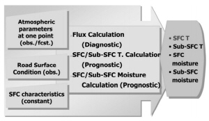
The prognostic model for the prediction of the road surface temperature is developed using the surface energy balance theory. This model tends to calculate the several micro-meteorologica variables, such as sensible heat flux, latent heat flux, ground heat flux, wind stress, and friction temperature (Fig. 1).

2. Model Description

2.1 Surface fluxes

The turbulent scales, such as friction velocity and friction temperature , are usually computed iteratively starting form neutral values. However, this method is computationally time consuming. An analytical approach is suggested by Garratt (1992) with the use of the bulk Richardson number and by Park (1994) in his surface parameterization.

The bulk transfer relation for surface fluxes is given by

 (1)

 (2)

where and are drag coefficients for momentum and heat in neutral stability, and are stability parameters that are the function of the bulk Richardson number for momentum, geat, and substring and represent each air and ground level.

2.2 Latent heat flux and evaporation

For evaporation calculations, soil moisture is required. Soil moisture levels are usually obtained through the bucket method or the force-restore method. One of the disadvantages of bucket method is that evaporation does not respond rapidly to short-period occurrences or pre-cipitation. In the case of two-layer scheme (force-restore method), a thin soil surface layer volumetric moisture content and the bulk layer volumetric moisture content are represented (Noilhan and Planton, 1989) by

   (3)

(4)

with

  (5)

where P is the precipitation rate, the evaporation at the soil surface, the snow-melt, the density of snow, R the run off, the transpiration rate, and are constants which depend upon soil types (Noilhan and Platon, 1989). is the intercepted rainfall by the canopy. For a bare ground and for a canopy, rain must first fill a reservoir of water on a canopy (), so that

 (6)

When , the depth of water residing on the foliage, reaches , the maximum depth of it, rain will no longer be intercepted but can reach the ground as throughfall. The variable in Eq. (5) represents an equilibrium moisture content where the force of gravity balances capillary forces.

 The soil moisture content is relate to a scaling depth and a subsurface soil layer of a physical depth of . They are

 (7)

where is the thermal diffusivity of the soil.

The soil evaporation is found from,

 (8a)

Where is the potential evaporation from the ground estimated by the Penman - Monteith equation (Monteith, 1981), which is given by

 (8b)

Where the latent heat of evaporation, the saturation specific humidity, the gas constant, the air temperature, and , the humidity deficit.

2.3 Road surface temperature and Subsurface temperature

The prognostic equations for the road surface temperature and subsurface temperature are obtained from the force restore method proposed by Bhumralkar (1975) and Blackadar (1976). That is,

   (9)

 (10)

where is the road thermal coefficient, the heat storage rate and the time scale as 24 hour. The coefficient is given by,

 (11)

where and are thermal coefficient of soil and vege-tation system respectively. is assumed to be (Noilhan and Planton (1989)). For no vegetation system, (e.g. ), the coefficient equals to , thermal coefficient of soil system depends on both the soil texture and soil moisture.

This is estimated by,

 (12)

The thermal conductivity and volumetric heat capacity C vary with the volumetric moisture contents and matric potential . That is,

 (13)

where is in unit cm (McCumver, 1980 ; Pielke, 1984) and the matric potential is,

 (14)

where is the saturated moisture potential, and the saturated volumetric moisture contents and b the slope of retention curve on logarithmic graph.

The volumetric heat capacity C is expressed by the density of the road soil, the specific heat and the soil moisture contents.

The ground heat flux can be calculated by the surface energy budget conservation theory. That is,

 (15)

where is the sensible heat flux that is the function of friction velocity and friction temperature, the latent heat flux and the net radiation flux.

3. Verification of Model

To verify the developed model, its output was compared with the data from the German Weather Service (DWD), which utilizes the Energy Balance Model (EBM) based on the energy budget balance theory.

DWD’s EBM calculates the energy transfer through 21 sub-surface medium and classifies 160 types of the climato-logy for road condition. And 5 types of other road cha-racteristics are considered.

We carry out the simulation for the L857 region (Hanau) of Germany by using both DWD’s EBM and the developed model with the same initial conditions and period (November 2012～March 2013).

To compare the results of both models, the forecasted road surface temparatures of both models and the observed one are shown in Figs. 2 and 3.

The simulated results by using both models were very similar to each other and had a good match with the observed data. But the forecasted road surface temperature by using the developed model is about 1 K～2 K lower than that of DWD’s EBM. To find the cause of the under-estimation of the developed model, we checked the calculated several flux amounts. Major difference was that when the heat is transferred between the road surface and the subsurface layer, the response of the developed model (2-layer model) occurs more quickly than that of DWD’s EBM (multi-layer model). So, the minimum temperature is affected by the heat transfer rate.

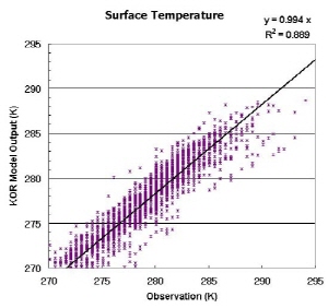
Two scatter diagrams and regression analysis results, which represent the relationship of the DWD’s EBM output, and those of the developed model and the observation, are shown at Fig. 3.

We can easily find that it is evident that the two model’s outputs and observed values are highly correlated, if the coefficient of determination R² and the slope of re-gression line are nearly unitary. But the developed model’s output has a little bit cold bias as already discussed in previous chapter.

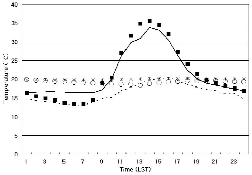
The developed model was run on 5 Oct., 2012, using the measurements of the KMA (Korea Meteorological Administration)’s pilot site which is located in Sindaebang- dong, Seoul and the model outputs are compared with the observations data. The pilot site is composed of both the meteorological tower and road sensor which can measure the road SFC/sub-SFC temperature and road condition.

The simulated results (Fig. 4) utilizing the developed model were compatible with the observed data, within the error of less than 2 K. At the same time, the time lag between air temperature and road surface temperature (about 3∼4 LST) was also well simulated by the model, as the measurement shows.

The numerical weather forecasting output from KMA/ MM5 was used as the synoptic input data, for running model. Because of the initial error of the MM5 output, the simulated road surface temperature and ground temperature showed the difference in values from the measurement. As a result, the quality of road surface condition was found to be dependent on the quality of the NWP, when we operated the Energy Balance Model for road weather prediction.

4. Conclusion

The prognostic model for the prediction of the road surface temperature is developed using the surface energy balance theory. And the developed model output is  compared with DWD’s EBM outputs and the pilot site’s observations to verify the developed model’s performance. The simulated results by using both model were very similar to each other and were compatible with the observed one. But the developed model underestimates the minimum road surface temperature rather than DWD’s EBM.

If the developed model is improved to have more subsurface layer, more accurate result will be produced.