1. Introduction

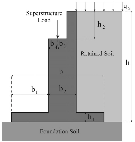
The recent development of the new American Association of State Highway and Transportation Officials Load and Resistance Factor Design (AASHTO LRFD 2013) for design of bridges focused on the superstructure components (Nowak, 1995 and 1999). Also, LRFD procedures for foundation desgin are already well established. However, studies on LRFD procedures for bridge substructures, particularly bridge abutments are relatively less established compared to those of superstructures and general foundation design criteria. Therefore, this study deals with the bridge abutment components. The objective of this study is to formulate the limit state functions, develop statistical models for load and resistance parameters, calculate the reliability indices for typical abutment components, and develop sensitivity functions for the load and resistance parameters. In this study, the reliability analyses are performed for a bridge abutment shown in Fig. 1, with dimensions of height, h = 3～12 m and base width, b = 0.4～-0.7h. Other dimensions are h₁ ≅ 0.1h, b₁ ≅ 0.1h, and b₂ ≅ 0.1h. The abutment structure analyzed is supported on spread footings. The retained soil is usually compacted (engineered) and its mechanical properties can be different from those of foundation soil.

2. Load Models

The load components typically required for the design and analysis of bridge abutments include dead load, DL, vertical earth pressure (EV), horizontal earth pressure (EH), vehicular live load (LL), and vehicular live load surcharge (LS). The statistical parameters of load used in this study are determined based on the available literature, test data, simulations, and engineering judgment.

For the dead load, the bias factor λ_DL = 1.00 and coefficient of variation COV_DL = 0.10. Similarly, for the soil unit weight, γ_S, the bias factor λ_γs = 1.00 and coefficient of variation COV_γs = 0.10 (Nowak 1999). The actual values of these parameters reported in literature are lower, however, the conservative values are consistent with the calibration of LRFD AASHTO Code (2013).

For vehicular live load bias factor λ_LL = 1.00 and coefficient of variation COV_LL = 0.10 (Nowak and Hong 1991, Nowak 1993). Live load surcharge is treated as a deterministic load.

The horizontal (lateral) earth pressure is a function of retained soil properties. The retained soil is usually compacted cohesionless soil. The effective friction angle, Φ_r, is the most important soil related parameter.

Load bearing capacity of foundation is a function of foundation soil properties. The most important soil parameter is the effective friction angle, Φ_f . It has been observed that the bias factor of Φ_f, λ_Φf increases with increasing value of Φ_f. The assumed relationship between λ_Φf and Φ_f is given in Table 1, based on conservative engineering judgment. Two test methods are considered: standard penetration test (SPT), and cone penetration test (CPT). CPT is recognized as a more accurate method.

The coefficients of variation of Φ_f in the available literature were calculated for various sets of test data. However, the cumulative distribution function (CDF) of Φ_f is non-normal, with a higher degree of variation at the upper tail of the distribution function. Therefore, in the reliability analysis, it is assumed that Φ_f is lognormally distributed.

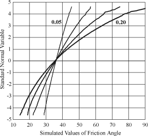
The reliability analysis is performed for a conservative case of design value of the friction angle Φ_f= 30°. CDF of Φ_f, being lognormal with the parameters, λ_Φf = 1.15 for CPT and λ_Φf = 1.20 for SPT, and four different values of COV_Φf = 0.05, 0.10, 0.15 and 0.20. The considered CDF are plotted on the normal probability paper in Fig. 2 for CPT, and Fig. 3 for SPT.

3. Limit States

The basic format of the limit state functions considered in this study is

g=R-Q (1)

where R is resistance (load carrying capacity), and Q is load effect. However, both R and Q are expressed in terms of parameters such as load components, material and soil properties, and dimensions.

Several limit states depending on structure types  were considered for inverted T bridge abutment:

∙ Bearing capacity of the foundation soil

∙ Sliding

For normal inverted T shape retaining walls, limit state function for overturning moment must be considered. However, in case of bridge abutment, there is governing magnitude of loads delievered from the superstructure, and the possibility of overturning failure is negligible. Therefore, for this study, overturning moment is not considered.

The limit state functions were based on the current design code (AASHTO LRFD 2013). For the bearing capacity limit state, the limit state function is

g_BC=q_ult-q_V (2)

where q_ult is bearing capacity of foundation soil, given as a function of soil Φ_f , footing shape, eccentricity of loading, and load inclination factor, and q_v is vertical stress in soil due to loads.

For the sliding limit state, the limit state function is

g_SL=Q_S-H (3)

where Q_s is sliding resistance and H is resultant horizontal load. Sliding resistance is a function of Φ_f and total vertical force applied to the foundation soil.

4. Reliability Analysis

The available reliability methods are presented in several publications (Nowak and Collins 2000). For the limit state functions (Eqs. 1-3) if g≥0, the structure is safe, otherwise it fails. The probability of failure, P_F , is equal to,

P_F=Prob(R-Q<0)=Prob(g<0) (4)

The reliability index, β, is defined as a function of P_F,

β=Φ^-1(P_F) (5)

where Φ^-1 is inverse standard normal distribution function.

In this study, reliability is calculated using Monte Carlo simulations because it is currently the most accurate and efficient approach (e.g., Elishakoff, 1999; Smith, 1986).  In practice, the accuracy of the Monte Carlo method is a function of the number of simulation runs. The new generation of computers allows for tens of thousands to millions of runs in seconds. Therefore, the computations can be performed very efficiently and accurately for any format of the limit state function and type of the random variables.

The only practical limitation to the Monte Carlo method is the accuracy of the assumptions used to formulate the limit state function and statistical parameters of the random variables (e.g., type of distribution function, bias factor and coefficient of variation).

Let the limit state function be g(X₁, …, X_n), where X₁, …, X_n are random variables and n is the number of simulations. The limit state function can be linear or non- linear. For each random variable, the cumulative distribution function (CDF) is needed, or at least value of the mean and coefficient of variation. If the type of CDF is not available, then a normal or lognormal distribution can be assumed. The reliability index is calculated by a random generation of values of the limit state function, and the analysis of the lower tail of the obtained CDF. The reliability analysis procedure used in this study includes the following steps:

1. Prepare input data: the limit state function with random variables representing the load and resistance parameters.  For each random variable, select the type of CDF and the basic parameters such as the bias factor and coefficient of variation.

2. Generate a value for each random variable X1, …, Xn using a random number generator. Actually, the computer generates uniformly distributed random numbers u1, …, un, and for each generated 0 ≤ u_i ≤ 1, the corresponding value of xi can be calculated from the following formula:

x_i=F^-1(u_i) (6)

3.where F^-1 is the inverse of the cumulative distribution function (CDF) of X_i.

4. Using the values of X₁, …, X_n, generated in Step 2, calculate value of the limit state function g(x₁, …, x_n), and save it in a file.  This value represents the safety margin.

5.Steps 2 and 3, to obtain the required number of values of g, e.g. 100,000.

6. Plot a cumulative distribution function of the obtained values of g. The probability of failure is equal to the value of CDF for g = 0. The determination of PF may require interpolation or extrapolation to extend the lower tail of the distribution of g. In some cases, an increased number of simulations may be required.

It can be more convenient to plot the CDF of g on the normal probability paper. The most important properties of the normal probability paper are that any normal distribution function is represented by a straight line, and any straight line represents a normal distribution function.  Therefore, data plotted on the normal probability paper can be more efficiently evaluated with regard to degree of variation and type of distribution. The construction and use of normal probability paper is presented in textbooks (e.g. Nowak and Collins, 2000).

In this study, the resulting cumulative distribution function of g was plotted on the normal probability scale to determine the reliability index.

5. Result of Reliability Analysis

The reliability analysis is performed for a representative bridge abutment. The maximum (and minimum) load factors specified by the AASHTO LRFD Code (2013) are as follows: 1.25/0.9 for DL, 1.50 for EH (active), 1.35/1.00 for EV, 1.75 for LL. For cohesionless soils the resistance factors are 0.45 for CPT and 0.35 for SPT for bearing capacity, 0.80 for sliding, and 1.00 for overturning.

For the abutment (CPT design), the geometry (deterministic) is as follows (see Fig. 1): h = 6 m, h₁ = 0.6 m, h₂ =1.8 m, b = 4.25 m, b₁ = 1.8 m, b₂ =0.9 m, b₃ = 0.3 m

The unit weight of concrete is γ_c = 23.5 kN/m³. Retained soil internal friction angle is considered as a lognormal random variable, with nominal value Φ_r= 30°. The weight of retained soil is γ_r = 18.1 kN/m³. The same values are assumed for foundation soil,  Φ_f= 30°, γ_f = 18.1 kN/m³.

The vehicle live load surcharge is assumed to be a uniformly distributed load, with q_s = 11.3 kN/m². Dead load from superstructure, DL = 117.4k N/m. Live load from superstructure, LL = 99 kN/m (Nowak 1999). Foundation soil and retained soil are treated as uncorrelated random variables. The computations were performed for four values of the coefficient of variation of Φ_S, COV_ΦS = 0.05, 0.10, 0.15 and 0.20.

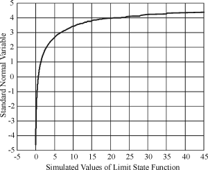
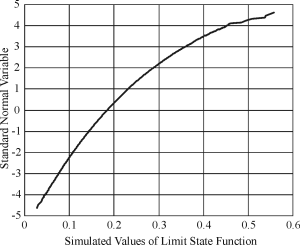
The simulated CDF of the safety margin, g, for COV_Φf = 0.10 (for both foundation soil and retained soil), is plotted on the normal probability paper in Fig. 4 for the bearing capacity, in Fig. 5 for sliding.

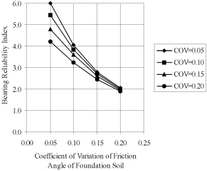
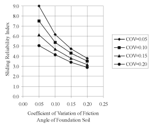
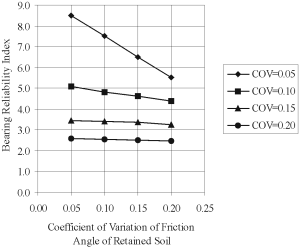
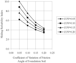
The reliability indices were also calculated for other values of load and resistance factors. The reliability indices calculated for other values of the coefficients of variation of Φf for foundation soil and retained soil are presented in Figures 6 and 7 for bearing and CPT, Figures 8 and 9 for sliding and CPT, Figures 10 and 11 for bearing and SPT, and Figures 12 and 13 for sliding and SPT.

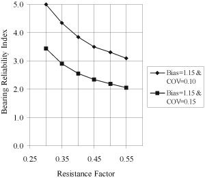
The relationship between the considered load factors related to earth pressure (horizontal and vertical) and reliability index is practically linear (within the practical range). It has been observed that friction angle of the soil, Φ_S, is the most important variable. The foundation soil is more important than retained soil. The reliability index is very sensitive with regard to the coefficient of variation of Φ_f. An increase of COV from 0.10 to 0.15 results in a decrease in the bearing reliability index by about 1.5. However, it was found that the reliability index can be considerably increased by reduction of the resistance factor, as shown in Fig. 14.

6. Conclusion

The objective of this study is to formulate the limit state functions, develop statistical models for load and resistance parameters, calculate the reliability indices for typical bridge abutment, and develop sensitivity functions for the load and resistance parameters.

The reliability indices were calculated using Monte Carlo analysis for a typical example of a bridge abutment. Two limit states are considered: bearing capacity and  sliding. The distribution of the safety margin, g, can be treated as a normal random variable for sliding and overturning, and it is closer to lognormal for the bearing capacity.

The effect of various parameters on the reliability index is evaluated. It has been observed that friction angle of the soil, Φ_S, is the most important variable. The foundation soil is more important than retained soil. The reliability index is very sensitive with regard to the coefficient of variation of Φ_f. An increase of COV from 0.10 to 0.15 results in a decrease in the bearing reliability index by about 1.5.

It was found that the bearing reliability index can be considerably increased by reduction of the bearing resistance factor, which indicates that the rational reassessment of bearing resistance factor is very important for economic design of bridge abutments.