1. Introduction

Standard penetration test (SPT) is one of the most simple and economical field tests used for ground investigation. Even though the test is known to include some uncertainties, the penetration resistance (N-value) has been extensively used for characterizing soil properties and preliminary foundation designs (Kulhawy and Mayne, 1990; Clayton, 1993). However, a general relationship between the SPT blow count and the cumulative penetration has rarely been investigated. In practice, field engineers just focus on the cumulative blow counts at the penetrations of 15, 30, and 45 cm, and then determine the N-value as the total blow counts from the last two penetration segments. In addition, field engineers often complete the test whenever the blow number in the last two segments reaches 50 at a penetration of less than 30 cm [N = 50/(<30)] in dense sand deposits. The premature completion is recommended in the UK practice (BS 1337-9, 1990). Differently, the US practice (ASTM D 1586, 2011) recommends that the test be completed if a total of 50 blows have been applied during any one of the three 0.15-m segments or a total of 100 blows have been applied from the beginning. The SPT is therefore still far from an international standard as the basic test procedure.

It is certain that the test is unreliable in gravelly soils where large particles may locally resists the penetration, leading to an unrealistically large value of N. In many cases of dense or cemented sandy soils, however, N > 50 reflects the true stiffness of the deposits at least for a preliminary design. The uncompleted test with N = 50/(<30) would give the underestimation of soil resistance. If the N value with 50/(< 30) is taken for a conservative design, design engineers might wonder how much the penetration resistance of such dense deposits is underes-timated. Therefore, a general relationship between the SPT blow count and the cumulative penetration is needed to elucidate the above concern.

There are a large number of studies on interpretation of the SPT N-value, its influence factors, and correlations between the value and soil properties. However, the behavior of the SPT during penetration has been rarely studied. Hettiarachchi and Brown (2009) introduced a basic concept of energy-based approach, and developed some formulas to estimate the effective friction angle (′) of sands and the undrained shear strength (su) of clays using SPT N60 value. Dung and Chung (2011) extended and improved the energy-based approach, and developed an equation (or energy-based equation) to simulate the relationship of the cumulative blow count versus cumulative penetration (hereafter termed as the penetration curve) during the SPT in sandy deposits.

This paper presents an improved energy-based equation to predict the SPT penetration curve, which allows a pre-maturely completed SPT N value to be extrapolated. To verify the proposed equation, a well-documented case record is used to compare between the measured and simulated penetration curves. The influence of some key input para-meters on the behavior of the penetration curve is discussed. In addition, a simple method for extrapolating the prematurely completed N values [i.e., N = 50/(<30)] is developed and the applied result is compared with that obtained using the energy-based equation.

2. Derivation of Pile Driving Equation

2.1 Basic principles and considerations

Pile-driving formula, which is in principle derived from energy balance approach, has been widely used for deter-mining the ultimate bearing capacity of driven piles (Poulos and Davis, 1980). The general mechanism of the approach is that the effective energy of each hammer blow is equal to the work mobilized so as to embed the pile to an incremental penetration at the ultimate resistance. Using this principle, the driving of the SPT sampler herein is conceptually modeled as that of a miniature open-ended steel pipe pile, which is to depict the penetration curve along the entire penetration depth in sandy soils.

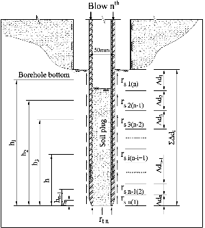
The plugging mechanism of the SPT sampler, in which the plug formation depends largely on the relative density and grading of the deposits, is rather complex. Especially, the plug formation is likely to be unpredictable in coarse and poorly graded deposits where the SPT N-value becomes much less reliable. To simplify the analysis, the following assumptions are taken into account: (i) soil is homogeneous within the test point and the high penetration resistance (N > 50) reflects the true stiffness of deposits; that is, the sampler is not locally resisted by large particles such as gravels or pebbles; (ii) the local shaft resistances acting on the inner walls of the sampler are not accounted for the total shaft resistance but for the base resistance; (iii) in-situ soil parameters (e.g., ′, K0) are approximately constant along the 45 cm penetration at each test point; (iv) for simplicity, energy that is spent to overcome dynamic resistance of soil is not considered. Fig. 1 shows a schematic diagram to represent the process of driving the SPT sampler at the nth blow, in which the symbols are detailed in the following sections.

2.2 Shaft resistance

The total shaft resistance up to the nth blow is generally given as:

 (1)

where rsi(j) = the unit shaft resistance (kPa) in the range of an increment Δdi subjected to j blows; Asi = 0.05πΔdi (m²) = the outer circumferential area of the sampler at the increment Δdi; K = the coefficient of lateral earth pressure [K= ηK0 = η(1- sin′)OCRsinφ′], where η = the factor taking into account the effect of increment of lateral earth pressure due to soil displacement; σ′v0 = the in-situ effective overburden pressure; and δ′ = the effective friction angle between sand and steel sampler surface (averagely taken as 2′/3). The thin hollow sampler often results in insignificant soil displacement during driving, so the horizontal stress incremental factor (η) should be close to unity. The factor η = 1.1 to 1.2 may be recommended for practical applications.

During pile driving (cyclic loading), the friction fatigue of soil elements surrounding the pile shaft has been well recognized (Randolph, 2003; Jardine et al. 2005; White and Lehane, 2004). This phenomenon leads to a reduction of shaft friction after each blow. The reduction of the shaft resistance at the increment Δdi is quantitatively represented by the factor βi(j) which is a function of the subjected blow number and the distance from the considering point to the pile base (White, 2005):

  (2)

where Ds = the sampler diameter (0.05 m), hi = the distance from the center of the increment Δdi to the base; and j = the number of blows at which the increment Δdi is experienced (j = n-i+1). It is noted that the maximum resistance is assumed to fully act on one pile diameter behind the pile base. Thus, the reduction factor βi(j) =1 if hi ≤ Ds.

2.3 Base resistance

The base resistance (Rtn) is probably the most difficult parameter in estimating pile bearing capacity, especially for open-ended piles. A number of methods for estimating the base resistance of driven open-ended piles were proposed (e.g., Jardine et al. 2005, Lehane et al. 2007); however, most of which relate the base resistance with CPT-qc value. To use basic in-situ soil parameters (e.g., ′, K0, σ′v0) and an independent solution of qc, the equation proposed by Paik and Salgado (2003) is adopted herein:

(3)

where rtn = the unit base resistance (kPa) at the nth blow, which theoretically increases with the decrease in the incremental filling ratio, IFRn; At = the cross-sectional area of the sampler’s base (approximately taken as 0.052π/4 m²); σ′h0 = the in-situ effective horizontal pressure; and = the coefficient that depends on the relative density at each test point. Paik and Salgado (1993) suggested that = 1 for dense sands, 0.6 for medium sands, and 0.25 for loose sands.

The most important parameter in Eq. (3) is the incremental filling ratio, IFRn, at the nth blow, which is not measured in routine performance of pile driving as well as of the SPT. Dung and Chung (2011) proposed a simple hyperbolic function as:

 (4)

where λ = a coefficient which varies according to the density of deposits (λ ≥ 0); m = the modified exponent (0 ≤ m ≤ 1). 

2.4 Energy balance equation

The energy (Eh) that delivers from hammer to the anvil at the nth blow (essentially the same for every blow) can be expressed as:

  (5)

where ETR = the energy transfer ratio; W = the hammer’s weight (kN); H = the hammer’s drop height (m). Note that the energy is the measured value right below the anvil.

As the stiffness of drill rods is much higher than that of the soil, the elastic deformation of the drill rods from each blow is significantly small compared with the penetration of the sampler into soil. Hence, such elastic deformation may be ignored in the analysis. The work (Es) done by the sampler to overcome the shaft resistance (Rsn) and toe resistance (Rtn) at the nth blow can then be expressed as:

(6)

where Δdn = the incremental penetration from the nth blow. The Rsn and Rtn values essentially increase with the increasing number of blows, which is because the pene-tration becomes deeper and soil plug gets denser.

Based on the energy conservation law, the equalization of the energies at the test depth gives:

 (7)

where CR = the correction factor for energy loss due to rod length (Skempton, 1986). By substituting Eqs. (1) and (3) for Eq. (7), a quadratic equation for the unknown Δdn is obtained.

(8a)

Or,

(8b)

2.5 Solving the balance equation

The incremental penetration Δdn (i.e., the positive root of Eq. 8b) from any nth blow can easily be obtained with the input parameters as follows: the in-situ soil parameters including σ′v0, ′, OCR, and ; the hyperbolic parameters for the IFR including m and λ; and the parameters related to the SPT equipment such as Ds, CR, W, H, and ETR. Note that after any Δdn (n ≥ 1) is obtained, the βi(j), rsi(j), and hi values at the previous increments (Δd1 to Δdn-1) are updated to obtain the next incremental penetration. This process is repeated until the cumulative penetration Σ(Δdi) reaches 45 cm.

3. Optimization of λ and m

Theoretically, the energy balance equation can be solved with a set of input parameters related to in-situ soil and SPT equipment and thereby a SPT penetration curve (consequently, the N-value) is obtained. However, the hyperbolic parameters (λ and m), which highly influence the variation of the penetration curve, are difficult to be measured or calculated from any routine SPT test. Thus, an attempt is made to optimize the λ and m using three data points obtained from the routine SPT: i.e., (n1,mea, d1), (n2,mea, d2), and (n3,mea, d3), where n1,mea is the measured blow counts at d1= 15 cm; n2,mea is the measured blow counts at d2 = 30 cm; and n3,mea is the measured blow counts at d3 = 45 cm. The iterative procedure to obtain the optimized values of m and λ can be briefly summarized as follows:

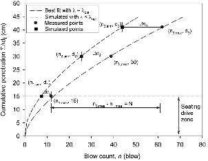
Iteration 1: With the first trial values m1 = 1.0 (the maximum) and λ1 = 0.0 (the minimum), a penetration curve is obtained by using Eq. (4) and Eq. (8b). The differences between the measured and simulated blow counts (Δni = ni,mea – ni,sim) at the three penetration levels are obtained, as graphically illustrated in Fig. 2. Then, the root mean squared error (RMSEm1,λ1) is defined as follows:

(9)

where ni,sim (i = 1, 2, 3) are the simulated blow counts corresponding to the d1, d2, and d3.

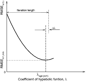
With any m value and λ1 = 0 (i.e., IFRn = 1.0), the same incremental penetration at every blow is obtained. The fact would possibly happen in extremely soft clays, not in sandy soils. The increase in λ (> 0) results in the increase in total blow count (n3,sim) and consequently the decrease in RMSE. Thus, the RMSE value at λ = 0 (for any m) is not expected as an optimized one. With the fixed value of m1 = 1, an iteration process is conducted by the increasing values of λ (λk = λk-1 + Δλ, where k = 2, 3, 4, …). As the increases, the RMSEm1,λ becomes smaller until it reaches a minimum value, and thereafter it again increases (Fig. 3). Once the optimized value of λ with the given m1 value (λ = λopt(m1)) is obtained, the iteration process is stopped. The minimum root mean squared error from m1 and λopt(m1) (RMSEm1,min) is quantitatively defined as:

(10)

Next Iterations: A similar iteration process is conducted for a different series of mi = mi-1-Δm, where Δm is a selected interval as small as 0.001. The m values of 1.0 to 0.0 are obtained with the index i of 2 to p = 1/Δm + 1. The minimum root mean square error RMSEmi,min for each mi value is obtained similar to the iteration 1. The optimal root mean square error RMSEopt is determined as the minimum value among the RMSEmi,min values with i = 1 to p.

 (11)

The values of m and λ corresponding to the RMSEopt are defined as the optimal ones and termed mopt and λopt, respectively. A Fortran code was developed for the iteration procedure.

4. Validation of the Proposed Method

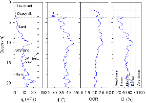
A well-documented experimental datum, which was con-ducted at a site named “Kidd2” of the Fraser River delta, south Vancouver, BC, Canada (Daniel, 2000), is used to verify the proposed method. The site consisted of loose to medium silty sand and sand. The groundwater level was around 2.0 m below the ground surface. Fig. 4 shows the qt profile and the corresponding profiles of ′, OCR and Dr interpreted from the CPTU data. More detailed information on geological conditions at the site was given by Daniel et al. (2003).

The SPT was experimentally performed at two locations (named as SPT9901 and SPT9904) by using a safety hammer of 640 N (144lb) with a drop height of 76 cm. A 0.61 m AW transducer rod was attached below the NW anvil rod of the safety hammer and the rest of the rod string consisted of 1.52 m AWJ rods. The split spoon dimensions were within ASTM standard. The number of blows required for each 2.54 cm (1 inch) of penetration was recorded. The effective energy transferred to the drill rods was monitored by using an HPA system.

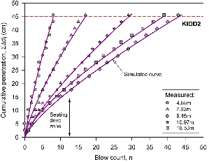
The increments Δm and Δλ were selected as 0.001 for the simulation. The energy transfer ratio (ETR) of 0.68 was averagely taken as the result obtained from the energy measurement test. The energy correction factor CR varied from 0.85 to 1.0 depending on test depth. In-situ soil input parameters based on CPT data and simulated outputs are given in Table 1. It appears that the simulated penetration curves match well with the measured ones (at the SPT9901 location), as typically shown in Fig. 5. The simulated N-value (Nsim) was just equal to or ± one blow of the measured one (Nmea). It can therefore be concluded that the proposed equation predicts the penetration curve effectively with the proper determination of the input parameters.

5. Discussion

5.1 Influence of λ and m

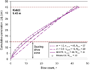
As shown previously, the behavior of the penetration curve significantly depends on the input parameters, especially on the hyperbolic parameters of λ and m. It is shown from Eq (4) that both λ and m control the variation of the IFR and thereafter the penetration curve. Theoretically, the increase in m at a specific depth (i.e., at the constant values of σ′v0 and Dr) should result in the decrease in λ and vice versa because the total required penetration (45 cm) is unchanged. An example of applying the theoretical equation to the measured data from the depth of 9.45 m of the Kidd2 site is shown in Fig. 6. The result shows that the best fit curve results in mopt = 0.580, λopt = 0.234 and Nsim = 34 blows. It also appears that as the m decreases from 1.0 (λopt = 0.097) to 0 (λopt = 0.942), the predicted curved plot gradually changes into an approximately straight line. As the m value approaches its upper and lower bounds (i.e., m = 1.0 and m = 0.0), the simulation tends to overestimate and underestimate the N-values by 37/33 and 29/33, respectively.

5.2 Influence of soil density

Soil density would affect the N-value as well as the penetration curve. To observe the density effect, a parametric study is conducted with a homogeneous and uniform sand layer: the bulk unit weight = 2.0 Mg/m³ and the groundwater table at 2.0 m below ground surface. At the depth of 20 m depth (σ′v0 = 220 kPa), five different values of corrected cone resistance (qt) were assigned to express various densities as given in Table 2. The density- dependent coefficient was properly assumed as shown in Table 2; i.e., the increases with the increase in Dr as practically proved in Table 1. With a typical value of λ for all the cases (i.e., λ = 0.2), the m values were also properly provided to reflect the fact that the m increases with the increasing density and in turn with the increasing curvature of the predicted curves.

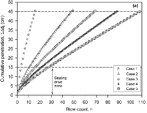
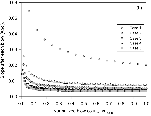
Fig. 7(a) shows the simulated penetration curves for the cases. It indicates that after passing the seating drive zone, the curves become approximately linear and the linearity is more pronounced with higher density. For a more closed evaluation, the relationship of the stepped slope of the curve at each blow (Δdi) versus normalized blow count (n/n3,sim) is depicted as shown in Fig. 7(b). As shown, the stepped slopes of the dense sands (cases 3 to 5) rapidly decrease at the early stage before they become constant; whereas the slope of the loose sand (case 1) continues to decrease until the final blow is reached. The key reason of such behavior may be attributed to the resistance that is caused by soil plug. It is inferred that the soil plug in dense sand becomes compacted more quickly than that in loose sand. When the soil plug is sufficiently compacted, the shaft and based resistances may steadily increase with the increasing blow counts and then lead to an approximately straight line at the latter parts of the curves. To prove this hypothesis, a comprehensive investigation is required with soil deposits where the soil density widely varies at a given depth.

5.3 Extrapolation of early completed SPT data 

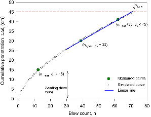
As previously mentioned, the routine SPT in dense sands is often completed before the total blow count of last two segments reaches 50 at the penetration of less than 30 cm [i.e., the SPT N = 50/(< 30)]. This fact will often result in an underestimate of the soil resistance. Thus, the extrapolation of the measured N value exceeding 50 is sometimes required. To achieve this purpose, the same procedure as used in the optimization section can be applied: for this case, n3,mea = n1,mea + 50 and d3 = 15 cm + dcomp should be adopted where dcomp = the completed distance (15 cm < dcomp < 30 cm). The simulation is continued until the cumulative penetration d reaches 45 cm. The extrapolated N-value, denoted as Next, is defined as the difference between n3,sim (the simulated blow count at d = 45 cm) and n1,mea, i.e., Next = n3,sim – n1,mea. Fig. 8 shows the simulated curve (open symbols) that fits the measured data points (solid symbols) and the target n3,sim value at 45 cm penetration.

Alternatively, Dung et al. (2011) suggested a simple method to determine the Next as follows:

Next=50×30/dcomp (12)

This simple equation implies that the three points, including the first point (n1,mea, d1), the third point (n3,mea = n1,mea + 50, d3 < 45 cm) and the extrapolated point, lie on the same linear line which approximately represents the penetration curve after passing the seating zone. However, this approximation may become less reliable because the early part of the experimental penetration curve is often more bent than that of the simulated curves (Fig. 6). Practically, soil beneath the bottom of borehole is subjected to stress relief and also to disturbance during boring and cleaning process, resulting in a lower density compared with that of the lower soil. Therefore, in this study, the linear extrapolation method can be revised by considering a straight line between the second point (n2,mea, d2) and the third point (n3,mea = n1,mea + 50, d3 < 45 cm) as shown in in Fig. 8. The line is extrapolated to the full penetration d = 45 cm and then the Next value can be determined. In general, the linear line would produce a slightly conservative Next value compared with that of the simulated curve because the stepped slope becomes progressively smaller as the blow counts further increases.   

6. Conclusions

A formulation was proposed to simulate the SPT penetra-tion curve in sandy deposits based on the energy balance approach. This formulation consists of three sets of input parameters: i.e., in-situ soil parameters (σ′v0, ′, K0 and ), hyperbolic parameters (m and λ), and SPT equipment- related parameters (Ds, CR, W, H, and ETR). Among them, the hyperbolic parameters significantly affected the curve. To achieve a better simulation, an iterative technique was used to optimize the values of m and λ (i.e., mopt and λopt) using three data points from the routine SPT. It was proven from a well-documented data that the simulated penetration curves obtained using the mopt and λopt match well with the measured ones. Thus, this formulation was applicable to extrapolating the prematurely completed SPT N value.

A parametric study indicated that at a given test point, the increase in m produces the increasing curved penetration curves and the increasing N-values. However, the predicted penetration curve became nearly straight for the portion of exceeding the seating drive zone (i.e., the cumulative penetration of 15 cm). This trend was more pronounced as soil density increases. Thus, it was possible to develop a simple and linear method to extrapolate a prematurely completed penetration curve in dense sands.