


1. 서 론
2. Rankine 토압론을 적용할 수 있는 뒷굽의 최소 길이와 이론적 파괴면 경사각
3. 한계해석법에 의한 주동토압 산정
4. 수치해석 결과
4.1 파괴면 경사각의 변
4.2 가상 연직면에 작용하는 배면마찰각, δ’
4.3 가상 연직면에 작용하는 주동토압
5. 결 론
1. 서 론
옹벽은 대표적인 토류구조물로 매우 큰 토압을 지지하는 케이슨안벽과 같은 항만구조물은 중력식 옹벽으로 설계하며 작은 토압에서는 캔틸레버 옹벽이 사용된다. 이러한 옹벽들의 안정성을 검토할 때, 한계평형법을 사용하여 벽면마찰력의 유무에 따라 Rankine 토압론 또는 Coulomb 토압론을 적용하고 있다. Coulomb 토압론은 파괴시 활동파괴면 사이의 흙쐐기에 대한 힘의 평형조건으로부터 옹벽에 작용하는 토압을 구하는 이론이다. 반면에 Rankine 토압론에서는 뒤채움 토사의 미소요소에 대하여 연직방향과 수평방향 두 평면에서 파괴시 각각 유발되는 응력상태를 Mohr-Coulomb 파괴규준식을 이용하여 토압계수를 구함으로써 토압을 구한다.
옹벽의 수평변위에 의해 뒤채움 토사가 파괴상태에 도달하면 옹벽 뒷채움재에서 내측(inward)과 외측(outward) 두 방향의 활동파괴면(slip failure planes)들이 발생하게 된다. Fig. 1(a)와 같이 사질토로 뒷채움한 캔틸레버 옹벽의 뒷굽이 충분히 긴 경우, 전단영역이 옹벽 벽체의 간섭에서 벗어나 활동파괴면의 형상에 영향을 주지 않는다. 따라서 뒷굽 끝단에서의 가상 연직면( )에 작용하는 토압을 산정할 때 Rankine 토압론을 적용하는 것이 이론적으로 문제가 되지 않는다(Terzaghi, 1943; Teng, 1962). 그러나 Fig. 1(b)와 같이 뒷굽의 길이가 충분하지 않아 내측 파괴면(
 )이 벽체와 만나면 전단영역이 영향을 받게 되므로 내측 파괴면의 경사가 가파라지며, 상부 벽체(
 )에서 발생하는 마찰력의 영향으로 가상의 연직면(
 )에 작용하는 마찰각, δ’가 지표면 경사, β와 같지 않을 경우 이론적으로 Rankine 토압을 적용할 수 없다. 따라서 이와 같은 경우에는 Coulomb 토압을 사용하는 것이 타당하나, 그럼에도 불구하고 Rankine 토압을 사용하는 것은 그 결과가 안전측이기 때문이다. Barghouthi (1990)는 Coulomb 토압을 유도하는 방법과 유사하게 한계평형법(limit equilibrium method)을 사용하여, 뒷굽이 짧은 캔틸레버 옹벽 배후 흙쐐기의 내측파괴면과 외측파괴면 경사각을 반복해서 바꾸어가면서 최대 토압을 나타내는 파괴면 경사각과 토압을 힘의 다각형으로부터 각각 구하였다. Barghouthi(1990)는 단지 2종류의 뒷굽 길이, 한 종류의 벽면마찰각과 한 종류의 지표면 경사각에 대해서만 분석하므로써 Coulomb 토압에 대한 영향 인자를 분석하는데 한계가 있다. Greco(2001)는 이론적 파괴면 경사각을 사용하여 한계평형법으로 뒷굽이 짧은 캔틸레버 옹벽에 대한 주동토압을 구하는 방법을 제안하였다. Yoo(2017)은 뒷채움 지표경사가 수평한 케이슨 안벽에서 바닥판이 돌출한 경우에 작용하는 토압을 한계해석법(limit analysis method)으로 구하였다. 한계해석법은 파괴시 발생하는 토체의 변위를 고려하여 파괴토체가 활동하면서 한 일과 이에 따라 옹벽이 움직이면서 한 일을 구하고 활동파괴면(토체와 원지반, 토체와 옹벽 사이의 활동면)을 따라 소모된 에너지를 각각 구하여 토압을 구하는 이론이다. 이때 파괴토체와 이에 상응하는 활동파괴면의 형상은 다양하게 가정한 파괴토체에 의해 발생하는 일과 소모되는 에너지의 양이 가장 작은 경우에 의해 결정된다(Chen, 1975). 따라서 다양한 파괴토체를 가정하기 위해서는 컴퓨터에 의한 시산법이 사용된다.

본 연구에서는 Fig. 1(b)와 같이 사질토로 뒷채움하고 지표면이 경사진 캔틸레버 옹벽에서 뒷굽 길이에 따라 흙쐐기의 자중, 옹벽의 벽체, 내측 파괴면, 외측 파괴면에 작용하는 힘을 한계해석법으로 구하였다. 이로부터 뒷굽 길이가 옹벽 배후에서 발생하는 파괴면의 경사각, 가상의 연직면에 작용하는 주동토압과 마찰각 등에 미치는 영향을 분석하였다. 본 연구에서는 옹벽 벽체에 작용하는 마찰각을 “벽면마찰각” δ로 표시하며, 뒷굽 끝단 연직면에 작용하는 마찰각을 “배면마찰각” δ‘로 표시한다.
2. Rankine 토압론을 적용할 수 있는 뒷굽의 최소 길이와 이론적 파괴면 경사각
본 연구에서 뒷굽길이가 짧다 또는 길다함은 뒷굽길이( )가 아래식의
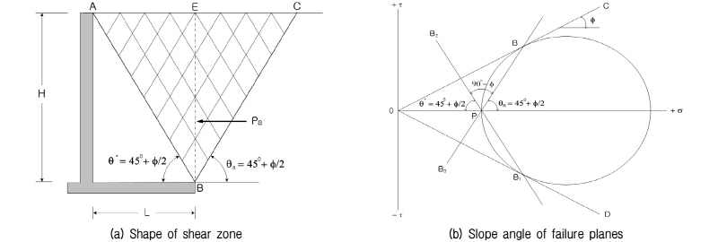
  보다 작거나 긴 경우를 말한다. 뒤채움 토사의 지표면이 수평한 경우에는 Fig. 2에 나타낸 바와 같이, 이론적으로 내측 파괴면(
 ) 경사각,
  와 외측 파괴면(
 ) 경사각,
  는 최대주응력면 또는 수평면과 45°+
 의 각도를 이루며, 그 값은 식 (1)과 같다. 따라서 뒷굽의 최소 길이,
  는 식 (2)와 같으며, Fig. 2(a)와 같은 조건이다.
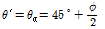 (1)
(1)
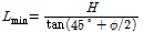 (2)
(2)
뒤채움 토사의 지표면이 경사진 경우에도 Fig. 3(b)에 나타낸 바와 같이,  와
와  는 최대주응력면(
 )과 각각 45°+
 의 각도를 이룬다. 지표면이 경사짐에 따라 최대주응력면이
  만큼 회전하므로,
  는 수평면과 45°+
 +
+ ,
,  는 수평면과 45°+
 -
- 의 각도를 이루며, 그 값은 각각 식 (3)과 식 (4)와 같다. 따라서 뒷굽의 최소 길이,
  는 식 (5)와 같으며, Fig. 3(a)와 같은 조건이다.

 (3)
(3)
 (4)
(4)

 (5)
(5)
여기서,  는 Fig. 3(c)에 도시한 바와 같이 구할 수 있다.
  ,
,  ,
,  는 이등변삼각형이므로,
∠EPF=∠PFC= , ∠EPC=2
 =∠PEC=λ-β 이다. 따라서
 이다. 한편
  에서
에서 
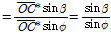 이므로
이므로  이다.
이다.
식 (1), (3), (4)에서 알 수 있듯이 이론적 파괴면 경사각은 벽면마찰각,  의 영향을 받지 않는다.
3. 한계해석법에 의한 주동토압 산정
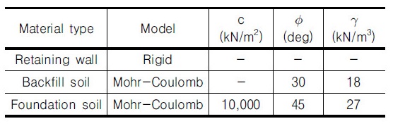
토압을 구할 때 한계평형법(LEM)은 옹벽 배후에서 발생하는 파괴면을 직선으로 단순화하여 만들어지는 흙쐐기에 대하여 힘의 평형조건을 만족시킴으로써 정역학적으로 문제를 해결하는 방법인 반면에, 한계해석법(LAM)에서는 한계평형법에서 고려하지 않은 변형에 대한 적합조건을 고려한다(Chen, 1975). 한계해석법을 적용함에 있어 이전에는 비교적 단순한 형상을 갖는 문제에 대해서만 한정된 갯수의 활동면을 가정하였다. 최근에는 이러한 문제점을 극복하기 위하여 DLO(Discontinity Layout Optimization) 기법(Smith et al., 2007)을 적용함으로써 복잡한 형상의 문제들에 대해서도 거의 무제한의 활동면들을 가정하여 해석결과의 정밀도를 획기적으로 제고할 수 있게 되었다. 본 연구에서는 Fig. 4(a)와 같이 파괴시 최소한의 에너지로 파괴에 이르도록 임의 활동면들의 방향성을 효율적으로 선택함으로써 파괴토체를 여러 개로 나누어 극한하중을 결정하는 DLO기법을 사용하는 한계해석법을 사용하였다. 뒷굽을 갖는 캔틸레버 옹벽을 Fig. 4(b)와 같이 모델링하였으며, 구성 모델의 물성값을 Table 1에 요약하였다. Table 1에서 캔틸레버 옹벽은 토압에 의해 변형되지 않는 강체로 가정하였으며, 기초 지반과 뒤채움 토사는 Mohr-Coulomb 파괴 모델을 따르며, 기초 지반은 지지력이 충분한 암반으로, 그리고 뒤채움 토사는 일반적인 모래로 가정하였다.

뒷굽의 길이가 토압에 미치는 영향을 분석하기 위하여, 뒷굽길이(L)와 옹벽높이(H)의 비( )를 0.1~
 까지, 뒤채움 지표면의 경사(
 )를 0°, 10°, 20°로, 그리고 벽면마찰각(δ)을 뒤채움토사의 내부마찰각의 1/2과 2/3로 즉, 15°와 20°로 각각 가정하여 수치해석하였으며, Table 2에 수치해석의 경우를 정리하였다. 본 수치해석에서는 옹벽높이를 5m로 가정하였으며, 옹벽 바닥판의 두께가 토압에 미치는 영향을 최소화하기 위하여 옹벽구조물을 강체로 그리고 두께를 1mm로 가정하였다.

4. 수치해석 결과
4.1 파괴면 경사각의 변화
Table 2의 수치해석결과 중에서 대표적으로 지표면 경사각이 10°이며 벽면마찰각이 15°인 경우에 대하여 뒷굽의 상대길이가 각각 0.0, 0.1, 0.2, 0.3, 0.4, 0.463 일 때 뒤채움 토사에서 발생하는 내측 및 외측 파괴면들을 Fig. 5에 나타내었다. 지표면 경사각과 벽면마찰각에 따라 해석된 내측 파괴면 경사각( ), 외측 파괴면 경사각(
 ), 이론적 파괴면 경사각을 Tables 3~5에 그리고 Fig. 6과 Fig. 7에 각각 나타내었다. 표와 그림에서 이론 파괴면 경사각을 “Theory”로 표현하였다.
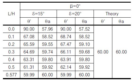


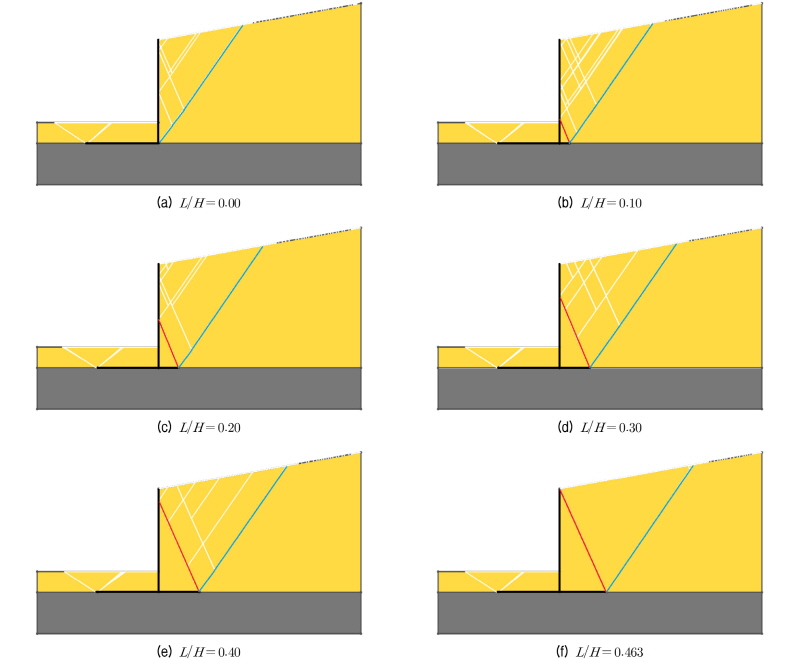
수치해석결과에 의하면, 뒷굽길이가 짧아질수록 내측 파괴면 상부의 옹벽 벽체(Fig. 1(b)에서  구간)에서 유발되는 마찰력의 영향을 크게 받아 내측 파괴면의 경사각이 Fig. 6에 나타낸 바와 같이 식 (3)에서 구한 이론 경사각보다 증가하나, 뒷굽길이가 길어질수록 벽면마찰력의 영향이 감소하여 식 (3)의 이론 경사각에 근접하며, 뒷굽의 길이가 최소길이(
 )이상이 되면 식 (3)의 이론 경사각과 같아지는 것으로 확인되었다. 뒷굽길이가 짧아질수록 내측파괴면의 경사각이 이론 경사각보다 크게 나타나는 경향은 뒤채움 지표면 경사각이 작을수록 그리고 벽면마찰각이 클수록 뚜렷하였다. 그러나 Fig. 6(c)에 나타낸 바와 같이 벽면마찰각이 지표면 경사각과 같을 경우(Rankine 토압 상태)에는 내측파괴면 경사각이 이론 경사각과 동일하며, 지표면 경사각보다 작을 경우에는 이론 경사각보다 작게 나타났다. 반면에, 옹벽 벽체와 멀리 떨어져 옹벽 벽체의 영향을 거의 받지 않는 외측 파괴면의 경사각은 Fig. 7에 나타낸 바와 같이 지표면 경사각이 수평하며
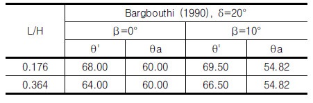
  <0.3 이내의 경우를 제외하면 식 (4)의 이론 경사각과 거의 같았다. Barghouthi(1990)가 한계평형법으로 구한 계산결과(Table 6, Fig. 6, Fig. 7 참조)는 본 연구결과와 잘 일치함을 보였다.


4.2 가상 연직면에 작용하는 배면마찰각, δ’
수치해석결과로부터 뒷굽 끝단에서의 가상 연직면(Fig. 1(b)에서  )에 작용하는 수평토압과 연직토압을 분리해내기 위하여 Fig. 1(b)를 Fig. 8과 같이 재구성하였다. Fig. 8(b)의 자유물체도에 나타낸 바와 같이 수치해석에서 파괴시 내측 파괴면 상부의 뒤채움 자중(
 ), 옹벽의 벽체에 작용하는 힘(
 ), 내측 파괴면에 작용하는 힘(
 )으로부터 가상 연직면에 작용하는 수평토압(
 )과 연직토압(
 )을 식 (6)과 식 (7)을 사용하여 각각 산정하였다. 이 수평토압과 연직토압의 합력(식 (9))이 가상 연직면에 작용하는 주동토압이다. 가상연직면에 대하여 수평토압은 수직력, 그리고 연직토압은 전단력에 해당하므로, 이들의 비는 가상연직면에 작용하는 배면마찰각,
  이라고 할 수 있다. 따라서 식 (8)을 사용하여 가상연직면에 작용하는 배면마찰각을 산정하였다. 그 산정 결과를 지표면 경사각,
  = 0°, 10°, 20°, 벽면마찰각,
  = 15°, 20°인 경우에 뒷굽의 상대길이에 따라 분석하여 부록 A에 각각 수록하였으며, Table 7과 Fig. 9에 그 분석결과를 요약하였다. 한편 Barghouthi(1990)가 한계평형법으로 구한 계산결과(Table 7 참조) 또한 본 연구결과와 잘 일치함을 보였다.


 (6)
(6)
 (7)
(7)
 (8)
(8)
 (9)
(9)
Fig. 9에 의하면, 배면마찰각( )은 뒷굽 길이가 짧을수록 벽면마찰각(
 )에 근접하며, 뒷굽길이가 길수록 즉, 최소길이,
  에 가까워질수록 지표면 경사각(
 )에 수렴한다. 따라서 배면마찰각(
 )은 뒷굽 길이에 따라 벽면마찰각(
 )과 지표면 경사각(
 ) 사이의 값을 갖는다.

 on a imaginary vertical plane at the end of heel
또한 배면마찰각( )은 벽면마찰각(
 )이 증가할수록 증가하며, 뒷굽 길이가 짧을수록 그 증가폭은 크며 뒷굽 길이가 길어질수록 증가폭은 작다.
배면마찰각( )은 벽면마찰각(
 )과 지표면 경사각(
 ) 사이의 값을 가지므로, Fig. 9(a), (b)에 나타낸 바와 같이 지표면 경사각(
 )이 증가할수록 뒷굽 길이에 따라 변하는 배면마찰각(
 )의 변화폭(
 )은 감소한다. 지표면 경사각(
 = 20°)이 벽면마찰각(
 = 20°)과 같게 되면, Fig. 9(c)에 나타낸 바와 같이 배면마찰각(
 )의 변화폭(
 )이 0(영)이 되어 뒷굽 길이에 관계없이 배면마찰각(
 )은 지표면 경사각(
 )과 같게 된다. 이 경우가 Rankine 토압 상태이다. 지표면 경사각(
 = 20°)이 벽면마찰각(
 = 15°)보다 크게 되면, Fig. 9(c)에 나타낸 바와 같이 배면마찰각(
 )이 벽면마찰각(
 )보다 커지는 현상이 발생한다.
4.3 가상 연직면에 작용하는 주동토압
4.2절에서 구한 수평토압과 연직토압을 사용하여 식 (9)로부터 합력을 산정하였다. 이 합력은 가상 연직면에 작용하는 주동토압,  를 의미하며, 식 (10)으로 나타낼 수 있다. 따라서 가상연직면의 높이,
  와 뒤채움토사의 단위중량,
  을 사용하여 식 (11)로부터 한계해석법에 의한 주동토압계수,
  를 산정하였다. 또한 지표면 경사각,
  = 0°, 10°, 20°, 벽면마찰각,
  = 15°, 20°인 경우에 뒷굽의 상대길이(
 )에 따라 가상 연직면에 배면마찰각(
 )이 작용하는 경우의 Coulomb 주동토압계수(θ’ = 90°인 경우),
  와 단지 뒤채움토사의 내부마찰각과 지표면 경사각의 함수인 Rankine 주동토압계수,
  를 식 (12)와 식 (13)으로 각각 구하여 이들을 부록 A에 각각 수록하였다. 이들의 관계를 뒷굽길이/옹벽높이, L/H 비에 따라 Table 8과 Table 9에 요약하였으며, Fig. 10과 Fig. 11에 각각 나타내어 비교하었다.
 (10)
(10)
 (11)
(11)
 (12)
(12)
 (13)
(13)

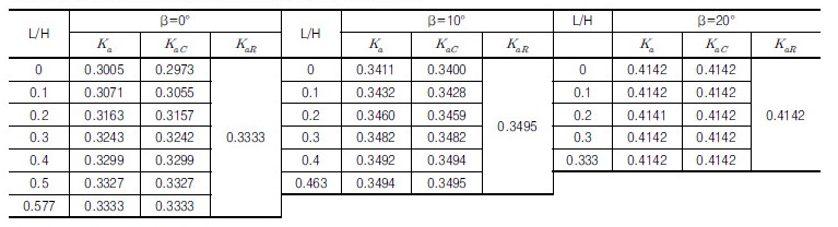

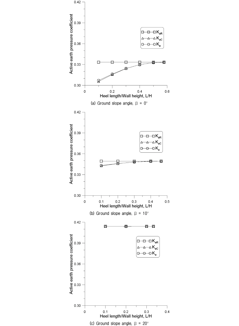
Table 8과 Table 9, 그리고 Fig. 10과 Fig. 11에 의하면, 한계해석법으로 구한 주동토압계수,  와 배면마찰각(
 )을 고려한 Coulomb 토압론으로 산정한 주동토압계수,
  가 거의 일치함을 알 수 있다. 토압계수는 뒷굽 길이가 짧을수록 Coulomb 토압계수와 같아지며, 뒷굽 길이가 길수록 Rankine 토압계수와 같아진다. 지표면 경사각(
 )이 벽면마찰각(
 )보다 클 경우, Coulomb 토압계수와 Rankine 토압계수와의 차이는 거의 발생하지 않는다. 그러나 지표면 경사가 수평한 경우에는 뒷굽의 길이가 짧아질수록 배면마찰각(
 )을 고려한 Coulomb 토압계수와 이를 무시한 Rankine 토압계수 사이에는 큰 차이가 발생한다. 또한 Fig. 12에 나타낸 바와 같이 토압계수는 벽면마찰각(
 )이 증가할수록 감소하였다. 뒷굽 길이에 따른 토압계수의 변화폭은 지표면 경사각(
 )가 증가할수록 감소하며, 이 현상은 4.2절에서 기술한 배면마찰각(
 )의 변화와 관계있다.

뒷굽이 짧고 지표면 경사각( )이 0°, 10°, 20°, 벽면마찰각,
  = 15°, 20°인 캔틸레버 옹벽에 내부마찰각이 30°인 사질토로 뒷채움할 경우, 뒷굽 끝단에서의 가상 연직면에 작용하는 주동토압을 다음 방법으로 구할 수 있다:
1)가상 연직면의 높이( )를 구한다.
2)뒷굽의 상대 길이( )에 따라 가상 연직면에 작용하는 배면마찰각(
 )을 지표면 경사각(
 )와 벽면마찰각(
 )를 고려하여 Table 7 또는 Fig. 9에서 구한다.
3)상기 2)항에서 구한 배면마찰각( )을 벽면마찰각(
 )으로 가정하고, 지표면 경사각(
 )와 벽면마찰각(
 )를 고려하여 θ’ = 90° 인 경우의 Coulomb 토압계수,
  를 식 (12)로 구한다.
4)가상 연직면(높이=H’)에 대한 Coulomb 주동토압( )을 식 (14)를 사용하여 산정한다.
 (14)
(14)
5. 결 론
뒷굽의 길이가 상대적으로 짧은 캔틸레버 옹벽에 대하여 한계해석법을 사용하여 옹벽 뒷굽 끝단 가상 연직면에 작용하는 토압에 대한 수치해석결과를 분석하여 얻은 결론은 다음과 같다.
(1)뒷굽길이가 짧아질수록 내측 파괴면의 경사각이 Mohr원에서 구한 이론경사각보다 증가하였으며, 이러한 경향은 벽면마찰각이 클수록, 그리고 뒷채움 지표면 경사각이 작을수록 크게 나타났다.
(2)가상 연직면에 작용하는 배면마찰각( )은 뒷굽길이가 짧을수록 벽면마찰각(
 )에 근접하며, 뒷굽길이가 길수록 즉, 최소길이,
  에 가까워질수록 지표면 경사각(
 )에 수렴하였다.
(3)뒷굽의 길이가 그 옹벽에 대한 최소길이( ) 이상으로 길다면, 어떠한 경우라도 가상 연직면에 대한 토압을 Rankine 토압론을 사용하여 구할 수 있음이 확인되었다.
(4)지표면 경사가 수평한 경우 뒷굽의 길이가 짧아질수록 배면마찰각( )을 고려한 Coulomb 토압과 이를 무시한 Rankine 토압 사이에는 큰 차이가 발생한다.
(5)본 연구결과인 뒷굽길이/옹벽높이 비( )와 뒷굽 끝단의 가상 연직면에 작용하는 배면마찰각(
 )과의 상관관계 도표로부터 가상 연직면에 작용하는 배면마찰각(
 )을 구하고 이를 사용하여 Coulomb 토압계수를 산정하면, 뒷굽이 짧고 지표면 경사각(
 )이 0°, 10°, 20°, 벽면마찰각,
  = 15°, 20°인 캔틸레버 옹벽에 내부마찰각이 30°인 사질토로 뒷채움할 경우, 뒷굽 끝단에서의 가상 연직면에 작용하는 주동토압을 구할 수 있다.
부 록 A
Table A.1 Friction angles and earth pressures on a imaginary vertical plane at the end of heel in case of β=0° and δ=15° 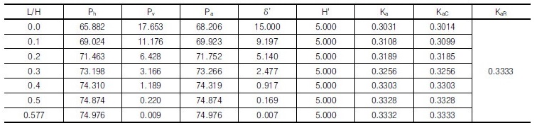 |
Table A.2 Friction angles and earth pressures on a imaginary vertical plane at the end of heel in case of β=0° and δ=20°  |
Table A.3 Friction angles and earth pressures on a imaginary vertical plane at the end of heel in case of β=10° and δ=15°  |
Table A.4 Friction angles and earth pressures on a imaginary vertical plane at the end of heel in case of β=10° and δ=20°
 |